
Abrasive Testing Data Logging: RPM and Pressure
A steady hiss from the airline. The muted rasp of a sander. The shop lights are still warming up when I pull on my respirator and set a fresh stack of mesh discs on the bench. Like most fabricators and finishers, I used to judge progress by sound and feel—when the pad tone lowers, when the dust plume changes shape, when the workpiece “grabs” differently. But the last round of panels told a frustrating story: same operator, similar substrate, identical discs—and visibly different finishes. One panel cut fast but glazed early. Another stayed cool but barely leveled orange peel. My notes were careful, but they weren’t enough. So I did what any test-obsessed engineer would do: I wired the tool.
Within an hour, I had a hall-effect pickup reading pad RPM, an in-line pressure transducer logging air supply, and a makeshift load rig to quantify downforce. That was my turning point. The difference between intuition and evidence is data, and in abrasive testing, two data streams—RPM and pressure—separate guesswork from control. Whether you’re qualifying new discs, dialing in robotic sanding paths, or troubleshooting burn-through, robust data logging is the shortest path to repeatability. It’s not glamorous. You won’t post photos of it. But you’ll sleep better when a spec holds across shifts and seasons.
This article is a field guide to data logging for RPM and pressure in abrasive workflows. I’ll compare sensor options, discuss sampling rates, show how to map force to finish metrics, and share workflows I’ve used to isolate variables cleanly. As a product engineer who lives in the gray zone between lab and shop floor, my goal is straightforward: make your abrasive testing tighter, faster, and more honest—backed by numbers you can defend.
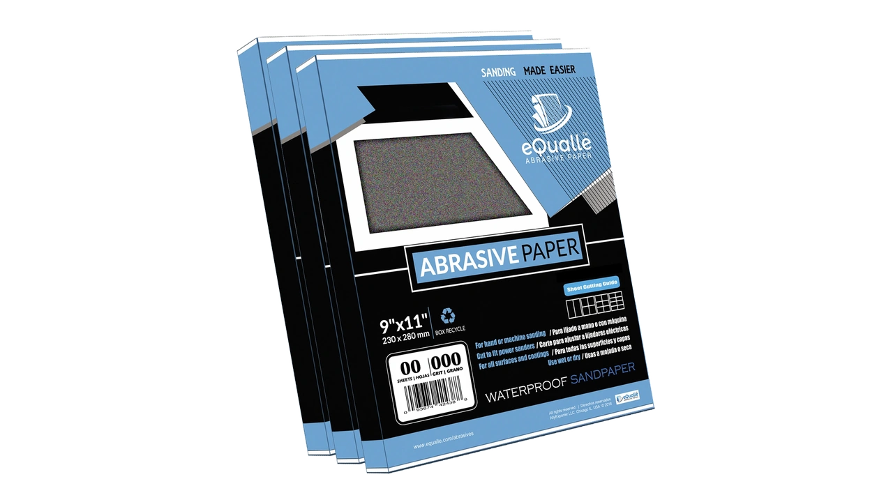
Quick Summary: Instrument RPM and pressure with the right sensors, sample fast enough, calibrate carefully, and tie the signals to cut rate and finish metrics for reliable abrasive testing.
Why RPM and Pressure Matter
In abrasion, energy delivery is king. Two knobs dominate that delivery at the tool: surface speed (set by RPM for a given pad diameter) and normal force (your applied pressure or robot downforce). At a fixed abrasive and substrate, these two parameters govern three outcomes you care about: material removal rate, surface temperature, and wear (both grain and binder).
- RPM controls tangential speed and the frequency of grain–workpiece impacts. Higher speed raises cutting events per unit time and can shift the regime from cutting to plowing if heat softens the binder or the substrate. For dual-action sanders, note that the effective path combines rotation and orbit; tracking both yields insight into scratch isotropy and loading behavior.
- Pressure sets contact stress. Too low and grains skate without engaging; too high and you embed grains or fracture the abrasive prematurely, accelerating wear and shedding. The sweet spot often emerges as a linear band where removal increases with force without exponential temperature rise.
Thermal effects blur the simple picture. Resin-bonded grains soften with heat; metals smear; wood fibers char. You’ll see a “knee” in removal-vs-pressure where temperature starts to dominate. That knee shifts with RPM, ventilation, and dust extraction efficiency. Measuring RPM and pressure concurrently lets you build maps: at 8,000 RPM and 30 N, the panel reaches 65°C after 45 seconds; at 11,000 RPM and 20 N, it stays below 50°C but cuts slower. With data, you choose tradeoffs intentionally.
Bench testers echo this logic. The Martindale abrasion method standardizes pressure and motion speeds (e.g., 23.8, 47.5, 71.3 rpm modes) to isolate material differences. Translating that rigor to hand or robotic sanding means logging the variables you can actually control. RPM and pressure aren’t the whole story, but they are the controllable majority—and the most cost-effective to measure with precision.
Sensor Stack and Logger Options
A practical instrumentation stack for sanding or grinding has three layers: sensing, acquisition, and power/packaging. Each choice affects signal quality, reliability, and operator burden.
Sensing RPM:
- Hall-effect or magnetoresistive pickup: Attach a small magnet to the pad hub or spindle; mount the sensor on a 3D-printed bracket. Pros: robust to dust, simple digital output. Cons: requires magnet placement, which may be tricky on sealed pads.
- Optical reflective or slotted encoder: Apply reflective tape to the rotating face or use an interrupter disk. Pros: high resolution. Cons: sensitive to dust and alignment; better on test rigs than in-shop.
- Motor current proxy: For brushed DC tools, armature current correlates with torque but only loosely with speed under varying load. Use cautiously and only after correlating to a true RPM reference.
- IMU-based estimation: Mount a small accelerometer/gyro on the body; derive dominant frequency. Works for orbital frequencies; less accurate for true RPM without careful calibration.
Sensing pressure/force:
- Inline pneumatic pressure transducer: Measures line pressure at the tool inlet. Good for diagnosing supply variability; only an indirect proxy for downforce.
- Force-sensing resistor (FSR) or thin load cell under the handle or backing pad: Direct measure of applied normal force. FSRs are thin but drift with temperature and load cycles; miniature load cells with proper conditioning are more stable.
- Torque/force sensor at robotic wrist: For automated systems, a 6-axis F/T sensor gives the cleanest normal-force channel, independent of supply pressure.
Acquisition and packaging:
- Microcontroller with SD logging (e.g., ARM/Arduino-class) at 200–1,000 Hz with time-stamping is sufficient for RPM, pressure, and force. Add anti-alias filtering on analog channels and debounce on digital edges.
- Single-board computers (e.g., Raspberry Pi) offer easy networking and richer UI but add boot time and SD card fragility unless ruggedized.
- Industrial DAQ (cDAQ/CompactRIO-class) shines in high-channel-count test rigs and endurance tests but may be overkill for portable shop use.
Power and UX matter. A small LiPo pack can run a two-channel logger all day if you sample intelligently. Encapsulate boards, strain-relief every cable, and keep mass away from the operator’s fingertips—instrumentation that changes the grip will change the data.
Actionable tips:
- Use a luggage scale as a quick calibration tool for downforce: press the sander onto the scale to map handle reading to actual normal force.
- Sample RPM at least 10× the highest expected frequency component; for DA sanders at 12,000 RPM (200 Hz rotation) plus a 5 mm orbit (~200 Hz), 2 kHz sampling avoids aliasing.
- Low-pass filter pressure and force at 20–50 Hz; you want the operator’s macro changes, not grip micro-vibrations.
- Record a sync signal (e.g., trigger or “start pass” tap) to align multiple runs for comparison.
- Log environment: temperature, humidity, and vacuum CFM if available; they explain outliers later.
Instrumented abrasive testing workflows
To convert raw signals into decisions, design your abrasive testing like a miniature DOE with clear inputs, controlled conditions, and measurable outputs. Here’s a workflow I use for sanding discs, flap wheels, and nonwoven pads alike.
Define the question. Example: Which 150 mm mesh disc delivers the fastest level-sanding on high-build primer without clogging under typical shop conditions? Translate that into variables you’ll hold constant (substrate, primer cure time, dust extraction, pad hardness) and the two you’ll log (RPM, normal force).
Build the test article. Prepare identical panels. Weigh them to 10 mg resolution before and after each pass to quantify removed mass. If you can, measure surface roughness (Ra/Rz) and capture consistent images for scratch assessment. Mount your sensors: a hall-effect RPM pickup and either a thin load cell under the handle or a luggage scale for static force mapping you’ll apply in runs.
Script the passes. For each disc:
- 2 warm-up passes to seat the grain and stabilize temperature.
- 3 recorded passes of 30 s each, straight-line pattern with 50% overlap, vacuum on full.
- Target 9,000 RPM and 25 N; let the operator work naturally but keep a real-time bar/LED showing force within ±3 N.
Log at 1–2 kHz for RPM and 100–200 Hz for force/pressure. Annotate pass starts and any anomalies (edge catches, hose snag). After each pass, brush the disc; do not blow it with oil-contaminated air.
Calculate outputs. Removal rate (g/s), specific removal (g/J if you also log current/voltage), average force and RPM, and temperature rise if you instrument an IR spot. Graph removal vs time and track any downward slope indicating loading. Many discs show a two-phase curve: fast initial cut, then a steady-state rate.
Use the data to set practical limits. You might find Disc A cuts 20% faster at the same force but overheats above 10,000 RPM; Disc B is slower but stable across 7–11 kRPM. That turns into recommendations your team can follow without interpretation. According to a article, tribology instruments often pair controlled load with torque and speed to map friction and wear; the same pairing—load and speed—anchors shop-floor sanding tests to physics rather than feel.
Finally, store raw logs and computed KPIs with traceable IDs: disc lot, substrate batch, ambient conditions. Six months later, when a batch behaves oddly, you’ll be glad you can re-run the exact analysis pipeline.
Data models, KPIs, and visualization
Raw time series are noisy and hard to compare. Define a lean data model and a set of KPIs that summarize behavior without masking instability.
Data model (CSV or Parquet works fine):
- Header metadata: tool, pad size, disc spec, substrate, operator/robot program, vacuum CFM, ambient temp/humidity.
- Time series columns: timestamp (ms), RPM, force_N, line_pressure_kPa (optional), torque_AmpereProxy or current_A, temp_C (optional), sync_flag.
- Event markers: start_pass, end_pass, disc_change.
From these, compute:
- Average and standard deviation of RPM and force per pass; high variance signals poor technique or unstable regulation.
- Removal rate (g/s) and, if you log power, specific energy (J/g). Lower J/g at equal finish usually means sharper grains or better dust evacuation.
- Thermal slope (°C/s) during the first 10 s: a fast rise foreshadows binder softening and loading.
- Stall/drag events: detect dips in RPM >10% from setpoint; correlate with force spikes to diagnose operator-induced bogging vs supply pressure drops.
- Orbit frequency stability for DA tools: FFT the force or accelerometer channel to spot bearing wear or pad imbalance.
Visualizations that work:
- Force–RPM scatter colored by removal rate: a quick performance map.
- Control charts of RPM and force across passes: show process capability.
- Cumulative removal vs time: reveals loading inflection distinctly.
- Heatmaps for robotic jobs: position-tagged removal or roughness over large parts.
For robotics, integrate with the turnover package you already generate—flow, pressure, temperature, RPM, travel speed, inspection photos, and thickness summaries tied to position allow you to stitch abrasive performance to coating outcomes later. Even in manual shops, consistency improves when the operator can see a simple “in-band” indicator for force and speed while you collect the raw numbers behind the scenes.
Keep your KPI set small and decision-oriented. The point isn’t to admire graphs; it’s to choose discs, set tool limits, and train people faster.
Validation, calibration, and safety
The best logger is worthless without calibration. Start by establishing traceable references for each channel.
RPM:
- Use a handheld optical tach with reflective tape on the pad hub to generate a reference at multiple setpoints (e.g., 6, 8, 10, 12 kRPM). Cross-check your hall sensor counts per revolution and detect missed edges.
- If possible, strobe the pad to visually verify rotational speed and detect pad slip relative to spindle—not uncommon under high torque.
Force/pressure:
- Map handle or pad force to a known scale. A sturdy luggage scale is perfect: press the running or static tool onto the scale through a flat plate and record the relationship between your sensor reading and actual normal force from 5–50 N.
- Verify pneumatic transducers with a calibrated regulator or deadweight tester. Note hysteresis and temperature drift; compensate in software or in your uncertainty budget.
Sampling and timing:
- Check for aliasing by stepping RPM through a sweep while logging—if your computed RPM wobbles at fixed speed, increase sampling or improve edge detection.
- Synchronize multi-device logs with a physical tap or LED flash detectable by both systems; software clock sync alone often drifts more than you expect over 30–60 s.
Safety and ergonomics:
- Encapsulate electronics to IP54 or better; abrasive dust is conductive and abrasive by definition.
- Route cables away from moving parts; add strain relief at the sensor and housing ends.
- Keep additional mass low and centered; don’t place sensors where they change operator grip or balance. If it feels different, it cuts different.
Document everything. A one-page calibration sheet with dates, equipment, and residual errors turns “trust me” into “traceable.” Recalibrate after tool maintenance, pad changes, or sensor replacement. The cost is minimal compared to scrapping parts or chasing phantom problems caused by drift.
3M Net Abrasive — Video Guide
A helpful bench trial compares 3M’s latest net discs (C2 and Blue Net) head-to-head against competing meshes. The video runs controlled passes on coated panels and metals, focusing on cut rate, loading resistance, dust evacuation, and finish uniformity. You’ll see how open mesh structure and resin systems balance initial aggressiveness with sustained performance as the disc heats and clogs.
Video source: 3M Net Abrasive Testing
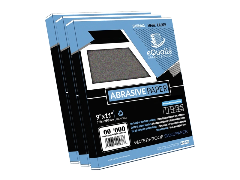
150 Grit Sandpaper Sheets (100-pack) — 9x11 in Silicon Carbide Abrasive for Wet or Dry Use — Versatile medium grit that transitions from shaping to smoothing. Works well between coats of finish or for preparing even surfaces prior to paint. (Professional Grade).
Frequently Asked Questions (FAQ)
Q: What sampling rates should I use for RPM and pressure? A: For RPM, sample at least 10× the highest expected frequency component—2 kHz comfortably captures 12,000 RPM rotation and orbital motion. For pressure or force, 100–200 Hz is usually sufficient since operator-induced changes are low frequency; apply a 20–50 Hz low-pass filter.
Q: Can line pressure stand in for applied downforce? A: Not reliably. Line pressure reflects supply and regulator behavior, not the normal force at the pad. Use a thin load cell or map applied handle force to actual downforce with a scale. Line pressure is useful for diagnosing air supply issues, but not as a direct surrogate for contact force.
Q: Do the tool’s built-in RPM readouts suffice? A: Treat them as setpoint indicators, not measurements. Many tools report unloaded motor speed; under load, pad RPM can drop 10–30%. Instrument the pad or spindle directly to capture true speed during cutting.
Q: What file format is best for storing logs? A: CSV is universal and fine for a handful of channels and sessions. If you scale up, consider Parquet with a simple metadata JSON to keep schemas consistent. The key is a clear data dictionary and consistent units (N, kPa, °C, RPM).
Q: Can a smartphone replace dedicated sensors? A: A phone’s IMU can estimate orbital frequency and detect gross changes, but it can’t directly read pad RPM or normal force with accuracy. Use it as a companion display or to annotate runs; for quantitative work, dedicated sensors remain necessary.